LS-DYNA: Implicit Quick-Start for Explicit Simulation Engineers
This is the 5th in a series of informal articles about one engineer’s usage of LS-DYNA to solve a variety of non-crash simulation problems. The first was on LS-DYNA: Observations on Implicit Analysis, the second was on LS-DYNA: Observations on Composite Modeling, the third was LS-DYNA: Observations on Explicit Meshing, and the fourth was LS-DYNA: Observations on Material Modeling
Most FEA work in the world is dominated by linear elastic stress and vibration analysis (implicit). The complexity varies tremendously within this realm and can be every bit as challenging as a highly nonlinear transient model (explicit). In the linear world, stress values are very sensitive to small changes in strain, and often take on even greater importance, since their values are used to verify the design margin of a structure or its fatigue life. Since the mission statements and analysis requirements between implicit and explicit analyses are different, one has to shift gears to move from one to the other. It is the focus of this short note to point out how a journeyman explicit simulation engineer can quickly and efficiently create implicit analyses from linear to nonlinear.
Where do I really start?
Not with this note. If you are seriously interested in implicit one should immediately start by reading Appendix P in the latest version of the Keyword Manual Vol. 1 and then proceed to DYNASupport.com and read the DYNAmore paper titled: “Some Guidelines for Implicit Analysis Using LS-DYNA.” Then, for examples and real-world scaling data on using implicit LS-DYNA, see Laird and Pathy “A Roadmap to Linear and Nonlinear Implicit Analysis with LS-DYNA” which can be found at DYNALook.com. However, if you are looking for a quick overview, please keep reading and we’ll try to boil it down as simply as possible.
High-Level Concepts
First off, we recommend using the latest release of MPP double-precision and sometimes, since implicit is changing so fast, the latest development version. It is on the cutting edge but today’s implicit cannot be compared with yesterday’s version. It truly changes that fast. Why MPP and double-precision? MPP scales better than SMP while double-precision is a necessity for clean convergence (i.e., nonlinear implicit). If you are hesitant about taking the plunge to MPP and are using Windows, we have a helpful webpage about LS-DYNA MPP usage.
Core Basics for Static Implicit
It just boils down to a few *CONTROL cards and carefully picking your element formulations. The following table provides our recommendations in alphabetical order that will ensure a robust nonlinear (material and geometric (large deformation and contact)) implicit stress analysis. If your focus is on linear implicit analysis, take a look at our paper: “A Roadmap to Linear…” since it covers all the tips and tricks and examples from this paper can be downloaded at DYNAExamples.com.
The alphabetical overview of what you need for nonlinear implicit analysis.
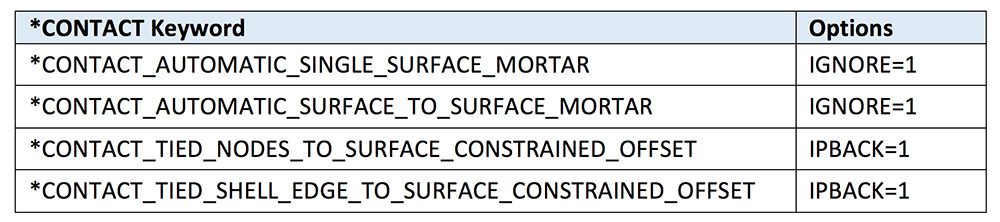
Contact
There really is only two recommended contact formulations for implicit. The advantage of _MORTAR contact is that it is very robust and the general formulation will also handle beam-on-beam contact. The only option that is recommended is that to set IGNORE=1 to handle small penetrations. Mortar is not restricted to implicit and works well in explicit, albeit a bit slow.
As for _TIED contact, we are really trying to narrow down the field to the most basic and most universal. For implicit, it is wise to avoid the use of springs or the penalty method whenever possible. Additionally, sometimes things don’t line up well and _OFFSET is needed. To address both of these requirements, one can use _CONSTRAINED_OFFSET with _NODES for tying solids to whatever and _SHELL_EDGE for tying beams and shells to whatever. Since rigid bodies are sometimes in the mix, if the option IPBACK=1 is added, the _TIED formulation is switched to a penalty method if a rigid body is detected. There is no harm that we know of using _OFFSET for a non-offset condition and likewise keeping the IPBACK=1 option turned-on even if no rigid bodies are present. The concept is to keep it simple and robust with minimum tweaking of basic Keyword Commands.
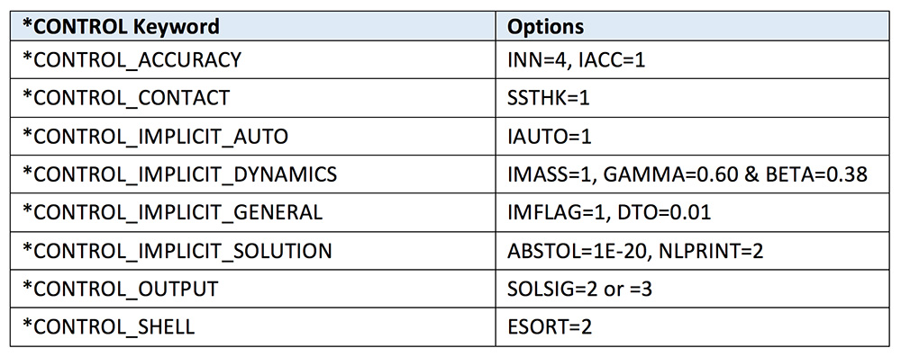
Control
This is my favorite section for setting up an implicit analysis since there are so many little pitfalls in the settings. In some cases, the cards have a bit of overlap with explicit settings. For example, the _ACCURACY card also includes the general explicit recommendation to set INN=4, so we carry this over to the implicit simulation for good measure. The setting IACC=1 does several little things and one should just read the manual (RTM). If one is using _SINGLE_SURFACE contact with shells, then it makes sense to also set SSTHK=1 (*CONTROL_CONTACT) to capture the true shell thicknesses.
One may notice that I don’t include *CONTROL_ENERGY in the setup. Since implicit isn’t worried about hourglass and if contact is used, SLNTEN is automatically calculated; hence, one less Keyword card to mess with.
The _IMPLICIT_AUTO setting is pretty much self-explanatory while the _IMPLICT_DYNAMICS setting is guaranteed to raise questions since we have stated that the overall *CONTROL settings are for a static implicit analysis and now we throw in_IMPLICIT_DYNAMICS? How can one resolve this obvious dilemma of turning a static analysis into a dynamic analysis? Well, it requires a bit of an explanation since this card represents one of the most important static implicit settings to obtain quick convergence in contact problems and often in large deformation problems (e.g., buckling). It has been our experience that at the start of a complex implicit analysis, there are several parts of the structure that require contact to be restrained (e.g., bolt preload). During initiation of the analysis, these structures are free to move and will generate warning messages from the solver since it is struggling to find convergence. A common work‑around by many nonlinear implicit codes is to apply a bit of numerical glue between the contacting surfaces during the first few iterations to stabilize the model (i.e., restrain floating parts). As the solution progresses, the stickiness between the contacts is reduced. This technique has its pros and cons but mostly cons since if friction is used, it can cause contacting faces to lock-up unexpectedly and change the load path. A better way is to avoid the use of such techniques and let the model behave as it would in the real world; that is, everything is dynamic in the real world. When a load is applied to a structure, no matter how slow, it is still dynamic. One will note that the option settings for _IMPLICIT_DYNAMICS is non-standard. By setting GAMMA=0.60 and BETA=0.38, the dynamic response is heavily damped. This hinders the structure’s dynamic response during load application and leads to a more static response of the structure as it moves and deforms under load. One concern in using this technique is the introduction of dynamic or inertia effects into a simulation that is designed to be static or free of dynamic effects. As mentioned, in the real world, all load applications are dynamic albeit some are faster than others. The idea of a slow, damped dynamic load application can be assessed by plotting the kinetic energy (KE) against the internal energy (IE). What we strive for is to maintain the KE below the IE during the simulation and should gradually decrease toward the end of the simulation. At the very end, it should be only a few percent of the IE. In this manner, we have a quantitative assurance that the simulation is behaving as a static analysis. In our experience, this approach leads to faster convergence for not only initially unstable contact analyses but also for material failure where element erosion can make the structure temporarily unstable, progressive failure of composites and buckling of structures. In short, we use _IMPLCIT_DYNAMICS (with GAMMA=0.60 and BETA=0.38) in every static, nonlinear implicit analysis model. A last little comment on using _IMPLICIT_DYNAMICS, your simulation is now aware of time and one can use BIRTH_DEATH options and if you want to and also just bury the dynamic behavior toward the end of the simulation (see the Keyword Card).
After that rather lengthy explanation of one Keyword card, everything else is rather mundane. For example, we have _IMPLICIT_GENERAL with a DTO=0.01 since we like to end our static implicit analyses at ENDTIME=1.0. The idea is to start easy and then let _AUTO ramp up the load as needed. As for the solver, we rarely ever touch the settings on _IMPLICIT_SOLUTION except to tighten up the convergence tolerance to ABSTOL=1e-20 and have it print out diagnostics with NLPRINT=2 (we’ll talk a bit about convergence failure later on under Troubleshooting). Since it is implicit and we are using fully integrated element formulations, we want to extrapolate the stresses (Superconvergent Patch Recovery) from the integration points out to the nodes. This is done using _OUTPUT with SOLSIG=2 or =3. Unfortunately this is only done for solid elements at this time. We are hoping that one day LSTC will add the same capability for shell elements. Currently, if one wants to view extrapolated shell stresses in LSPP, it requires the use of extrapolate. The last command automatically switches the element formulation for triangular elements from ELFORM=16 to ELFORM=17.
Database
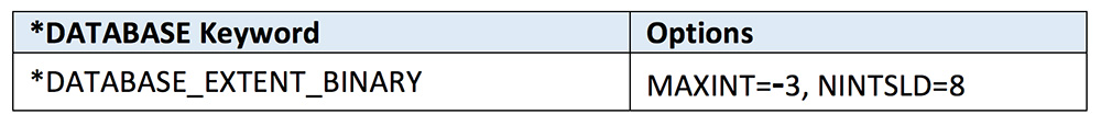
There is only one specialized command for implicit and it really isn’t specialized to implicit. It has to do with dumping out all the stresses from the full integration point set. For example, with MAXINT=-3 setting one gets all integration point stresses at the outermost NIP layers and at the midplane (if the recommended NIP=5 is used). Likewise, if NINTSLD=8, all integration point data is written out whether it is a brick or a tetrahedral. As for beams, that is a user choice as to what number of integration points to kick out using BEAMIP.
Section
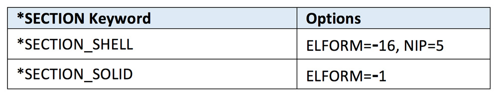
For isoparametric elements (which according to Ed Wilson (see www.edwilson.org) “The introduction of the isoparametric element formulation by Bruce Irons in 1968 was the single most significant contribution to the field of finite element analysis during the past 40 years”), one simply switches the element formulation to a fully integrated formulation. For shells, it is recommended to use the more advanced formulation ELFORM=-16 and for solids, the ELFORM=-1 does a nice job at reasonable numerical cost (see Tobias Erhart’s excellent work “Review of Solid Element Formulations in LS-DYNA”). Otherwise there is nothing special about setting up the definition. As with all isoparametric elements, one should not be too loose and fast with element quality. Good element quality always pays dividends in convergence and in pleasing stress results or in other words, if it looks good it is good. If one is interested in light discussion of the topic, take a look at “See Analysis Data’s True Colors” by Laird and Waterman.
Why Implicit?
For most of us, being a good simulation engineer is being skeptical of anything that looks too easy; that is, we just know that we are going to find challenges somewhere, somehow. Our experience has followed this dictum of struggling to obtain convergence, uncovering new, undocumented features and being perplexed more often than we like in the pursuit of a quality static nonlinear implicit solution. The model shown in Figure 1 was no exception and convergence was eventually obtained by not rushing the process and paying attention to mesh quality, contact behavior and using the absolute latest version of LS-DYNA MPP Double-Precision.
The model follows all the standard keywords as outlined above. It sounds so easy but what would trip us up is the usual silly modeling omissions where joints were not properly setup and would create mechanisms and greatly hinder convergence. With hindsight, one would always create pilot models of complicated sections and debug these sections first, but that would be too logical, we would rather suffer.
Figure 1: Manufacturing jig that is subjected to static triaxial loading
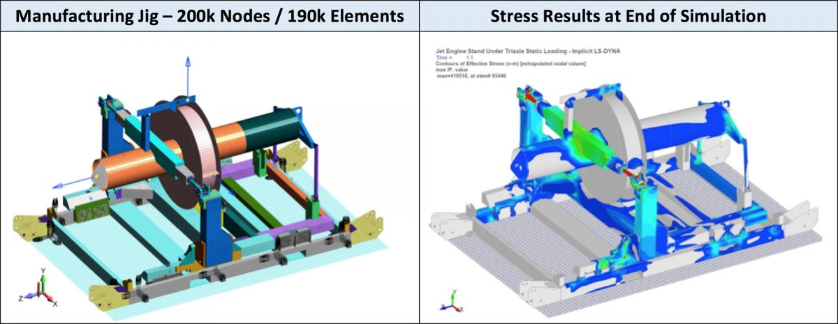
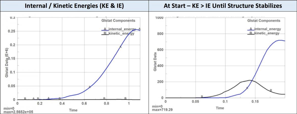
Some additional notes about the model is that the kinetic energy (KE) does exceed the internal energy (IE) at the start of the simulation. This can be expected since the structure is moving under the load (high KE) and the strains are minimal (low IE). Once the structure stabilizes, the IE rapidly shoots up. At the end of the simulation the load is held constant from 1.0 to 1.1 and the analysis settles to equilibrium.
One of the more useful implicit applications is for model preload prior to explicit. This is something we have done many times with composite structures to test firing of instrumented test munitions (see Figure 2). This is done as one analysis routine within LS-DYNA and not a start/stop/re-start routine but a seamless run from implicit to explicit.
Figure 2: US Army’s SCAT gun used to improve munition design

Troubleshooting
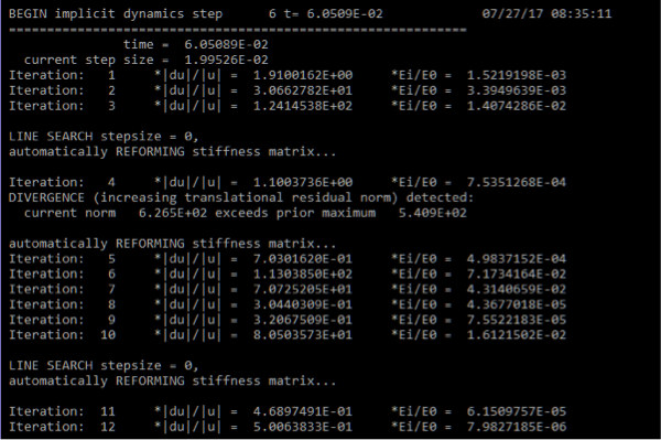
Although one hopes to read about some magic approach that will solve all your convergence issues, it doesn’t exist as far as we know. Figure 3 shows an example of an analysis running along doing the usual convergence dance. The report of |du|/|u| tells us about how the structure is physically moving and deforming. When this shoots up, it means that the structure is un-constrained, has buckled or is just loose. The other measure of Ei/Eo is the strain energy. If this shoots up, then one typically has a large plasticity issue where finding equilibrium is difficult.
Figure 3: LS-DYNA MPP Double-Precision analysis run with NLPRINT=2
Although one can recommend changing the number of equilibrium iterations prior to matrix reformulation or changing the line search method or adjusting the convergence tolerances, our experience with these practices has been dismal. What has worked for us is to tear apart the model and analyze sub-sections to determine why convergence is not occurring. What we like about the divide and conquer approach is that small models run quickly and lead to insights about why convergence is not occurring that can then be leveraged forward to future implicit simulations.
Another effective strategy that we have used to diagnose convergence problems is to contour the residual forces that are being calculated within an equilibrium iteration. This is done by setting D3ITCTL=1 in *CONTROL_IMPLICIT_SOLUTION and then RESPLT=1 in *DATABASE_EXTENT_BINARY. For more details, please read the most excellent Appendix P in the Keyword Manual Vol. 1.
Wrap-Up
Lest we not forget, the title of this blog is Quick-Start and it is far from comprehensive. The idea is just to open the door toward using the implicit solver and remove some of the fear, uncertainty and doubt (FUD) about getting started. It should also be mentioned that the LSTC support team does an outstanding job in supporting the implicit solver and you will not be left dangling.
Thank you for your interest and we would welcome any feedback that you might have on this article.