CFD Quiz
Welcome to our CFD quiz! Computational Fluid Dynamics can incorporate physics well beyond simple flow to include heat transfer, thermodynamics, multi-phase flow, and even structural-fluid interaction. This quiz will cover basic concepts of thermo-fluid engineering and present some more challenging questions for experienced CFD engineers that delve into the interesting intricacies of fluid flow modelling.
What unit does the Reynolds number have?
None, the Reynolds number is a dimensionless value
What is the difference between dynamic and kinematic viscosity?
Dynamic viscosity relates shearing stress to fluid motion and has the SI unit of Pa-s or the customary unit Centipoise (1cP = 0.001 Pa-s). The kinematic viscosity is the ratio of the dynamic viscosity to the density of the fluid, and has the SI unit of m2/s or the customary unit of Stokes (1St = 1 cm2/s).
You have gas in a contained volume that is heated from 300K to 500K. Does the density increase or decrease?
The density will stay the same as the volume is constant, and no mass is entering or leaving the enclosure. The pressure will increase with the higher temperatures
The volume an ideal gas will occupy at an equivalent pressure is proportional or inversely proportional to temperature?
The volume is proportional to temperature and will occupy a larger volume at a higher temperature, assuming the pressure remains the same.
In fluid boundary heat transfer, the Nusselt number describes what ratio? (Bonus: Who is it named after?)
The Nusselt number defines the ratio of total heat transfer at the boundary to the conductive heat transfer. With this ratio, you can define the heat transfer convective coefficient. This value was named after Ernst Kraft Wilhelm Nußelt.
For heated air at 150°F traveling down a circular duct, which flow rate definition would have the higher mean velocity: 200 CFM or 200 SCFM?
SCFM stands for Standard Cubic Feet per Minute, while CFM is the actual flow rate running down the duct. In the US, standard conditions are typically assessed at 68°F and 1 atmosphere, while this reference may be different for other places in the world. The important part, is that from the standard values for pressure and temperature (which will be lower than the problem statement), you can deduce a mass flow rate. When working back through the ideal gas law for the operating conditions, you will realize a lower density than standard conditions, which will result in a much higher actual flow rate than 200 CFM, resulting in higher mean velocities for 200 SCFM.
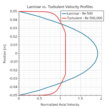
What are the characteristics of Laminar flow in a pipe?
Laminar flow consists of smooth parallel streamlines of velocity without the presence of mixing, local eddies, or random velocity fluctuations. Within a pipe, laminar flow will result in a parabolic velocity profile from the walls, whereas fully developed turbulent flow will have a flatter mean average velocity profile near the center.
When using a RANS turbulence model, what does the fluid velocity vector represent?
The fluid velocity vector from a RANS simulation will represent the time average or mean average of the velocity field. This value does not include instantaneous velocity fluctuations resulting from flow turbulence
What are the preferred combinations of flow boundary conditions for a CFD analysis
- Define equal values of mass flow inlet and mass flow outlet conditions
- Define mass flow inlet or velocity inlet with an outlet static pressure
- Define an inlet total pressure with an outlet mass flow rate or velocity
- Define an inlet total pressure with an outlet static pressure
Solution:
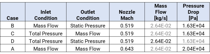
In most cases, choice B is the best combination of those listed, as it provides a combination of boundary conditions most compatible with the governing equations. Options C and D may also be good choices for particular conditions, but could lead to convergence issues in some cases. Option A should be avoided at all cost as it could lead to setup error issue, divergence, and provides no information on pressure, which is critical for state calculations.
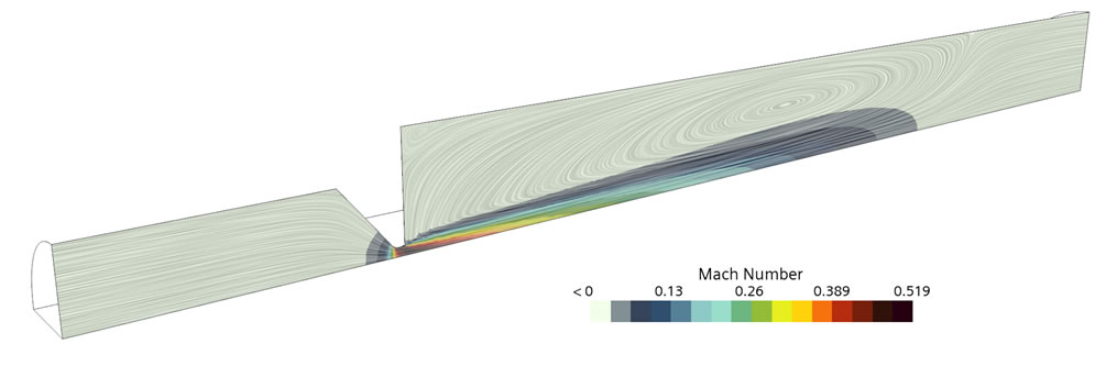
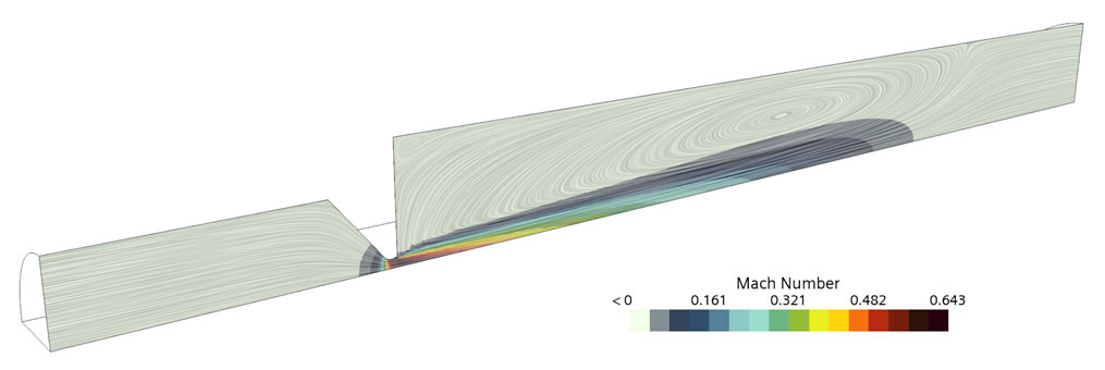
Let’s look at this quick example below of compressed air flowing through a nozzle. Cases B through D work well for this option and all provide repeatable results on mass flow, pressure drop, and peak Mach number achieved through the orifice. Option A provides wildly different results on peak Mach number and pressure drop. This is due to the fact that none of the boundary conditions provide a reference for pressure, so the solution must rely on the initial pressure conditions to float to a converged solution.
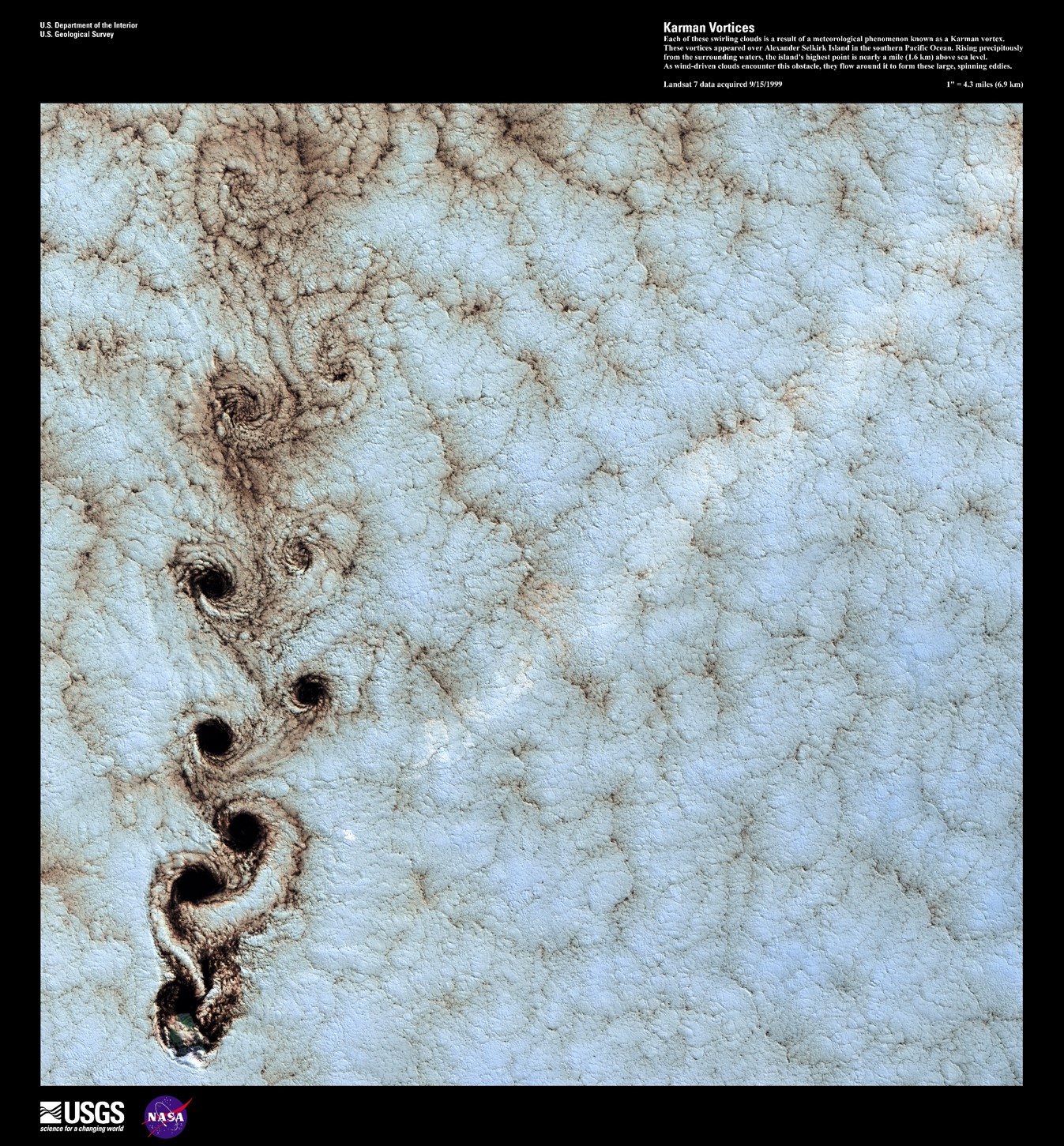
You have been assigned to characterize the flow around a bluff body. Your co-worker, who is an expert in structural simulation, suggests that you should take advantage of symmetry to reduce the computational effort. Should you follow his suggestion?
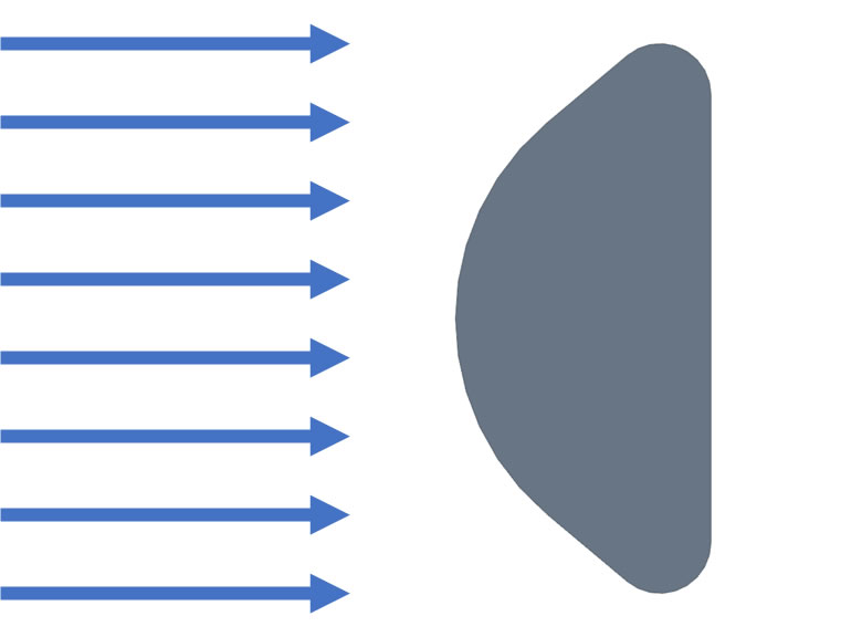
No:
This is a classic trap in fluid mechanics and CFD, where the geometry defining the flow path is symmetric, but the end result will not be. Exterior flows over bluff bodies or cylinders will induce wake zones and recirculation regions. In addition, the flow will also separate from the body at sharp angles or on the downstream side. These vortices that develop will not completely balance one another, inducing a transient phenomena known as vortex shedding. This is not a numerical artifact of the CFD solution, but a real and observed effect that can cause structural damage through modal coupling.
The example below shows two cases of flow over a bluff body where we apply a symmetry boundary at the midplane (top), and where we model the full span (bottom). The symmetry boundary forces the recirculation zone to be balanced and stabilizes the point of flow separation. Although this looks nice and neat, this would not reflect reality. With a full span model, we can observe the vortices coming off the rear end of the body, which are not symmetric.
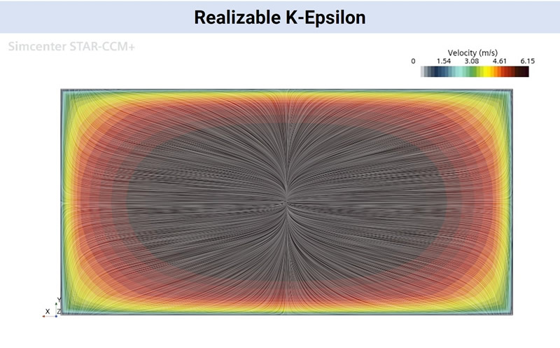
You are interested in modeling air flow through a square duct. You’d like the most accurate model to capture potential secondary flows. What RANS turbulence model should you choose and what are the potential pitfalls to watch out for?
- Realizable K-Epsilon
- K-Omega SST
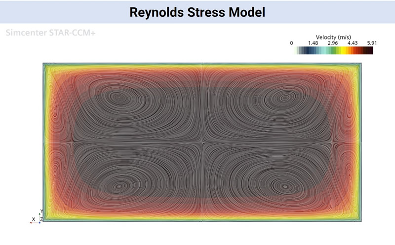
- Reynolds Stress
- Model Spalart-Allmaras
C will give you the most accurate model to capture potential secondary flow. Of the models listed, the Reynolds stress model is the only one to capture the anisotropic nature of turbulence and secondary flows. This model will add six additional equations to solve which will significantly increase computational effort and can lead to convergence challenges. You will need to ask yourself, just how important this additional level of detail is. In the example model below, the RKE model does not capture the well known secondary flow swirl that develops in rectangular ducts and underpredicts the pressure drop by more than 10%.
You have a high temperature low pressure application where you wish to simulate Nitrogen gas flow through a gap of 2.5 mm at a temperature of 1200 °C and absolute pressure of 5 Pa. Can you solve this problem with the Navier Stokes equations?
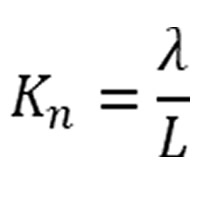
No. The Navier Stokes equations are only valid for continuum flow conditions. The low pressure conditions here require us to determine what flow regime we are in by evaluating the Knudsen number to determine flow rarefication. The Knudsen number is the ratio of the molecular mean free path, 𝜆, to the pertinent dimension, 𝐿, which is our gap dimension of 2.5 mm.
The molecular mean free path is the average distance traveled by a gas molecule between collisions and can be defined by the following relationship:
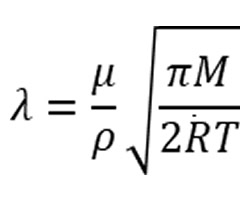
Where 𝜇 is the dynamic viscosity, 𝜌 is the gas density, 𝑅 ̅ is the universal gas constant, 𝑀 is the molecular mass, and 𝑇 is the gas temperature. From the Knudsen number, the various flow regimes are defined as follows:
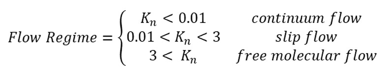
Based on the defined temperature, pressure, and gap from the problem, we calculate a Knudsen number of 3.5, which puts us in the free molecular flow regime.
For a Lagrangian-Eulerian multiphase particle flow analysis, what items must be considered to determine if you should use one-way or two-way coupling.
- Froude number
- Volume fraction of the Lagrangian phase
- Stokes number
- Particle shape
- TRICK QUESTION! ALWAYS USE 2-WAY COUPLING!
|
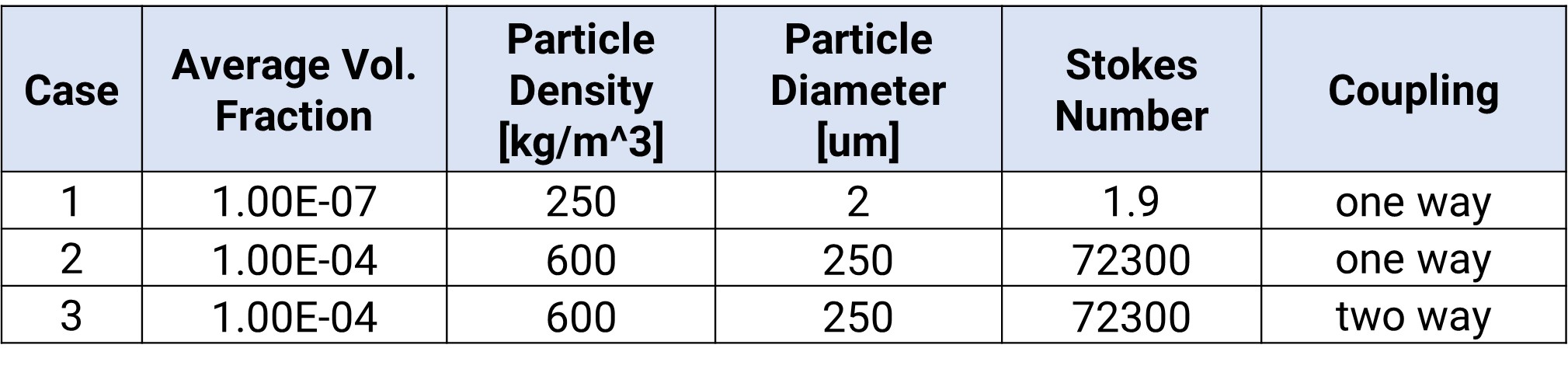
ANSWER; B and C The assumption of a one-way couple system is valid for cases where the dispersed Lagrangian phase will generally follow the flow of the continuous phase and have no significant impact on the continuous flow. This is valid for very low volume ratios (safely below 1e-6), but a second aspect to keep in mind is how well the particles will track the continuous flow path. If the particle is much denser than the fluid, and the particle momentum is not able to change as fast as the fluid direction, this can lead to local higher volume ratios and exchange of momentum between the particles and fluid. This effect can be determined by evaluating the Stokes number. An example case below shows wood dust particles in an exhaust duct with bends. For the first case with low volume fraction, smaller particle size, and lower density, the one-way coupling assumption is appropriate. For the next case, the higher density and diameter lead to a much larger Stokes number. In addition, with the higher particle volume fraction, we need to start considering two-way coupling. The larger and heavier particles with the higher Stokes value no longer follow the path of the fluid through the bends. The addition of two-way coupling to the model increases the accuracy of the particle paths and now accounts for the impact of the particles on the surrounding air flow. We see this in Case 3 with a tighter packing of the heavier particles as they travel through the bends.
|
n a meeting with your client, you show an image of water pressure down a length of pipe with a sudden expansion. The image shows the pressure is increasing in the direction of flow. The client questions your competence as a CFD simulation engineer. Does your client have a valid concern?
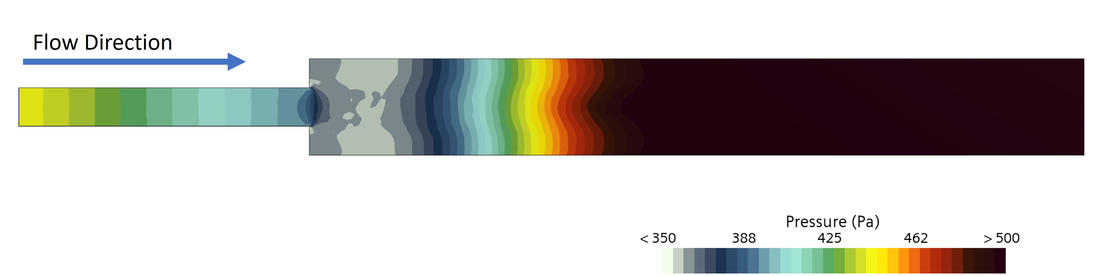
In the application used, Simcenter STAR-CCM+, the plotted working pressure is roughly equal to the static pressure (aside from a small turbulence effect and hydrostatic effects). Since there is no height change in the above problem, we can step back from CFD and look at the Bernoulli equation for flow down a streamline in the center of the pipe near the expansion (to ignore the pipe head-loss on either side):
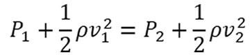
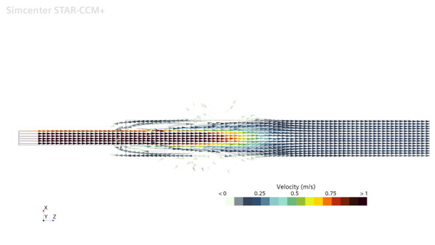
As the water is incompressible, the volumetric flow rate is constant throughout, so the velocity decreases through the expansion with the larger cross-sectional area. With the velocity after the expansion, 𝑣2, lower than the inlet, 𝑣1, The static pressure at 𝑃2 must be higher than 𝑃1 to balance the relationship. This is the culprit of why we have an unintuitive increase in pressure in the direction of flow.
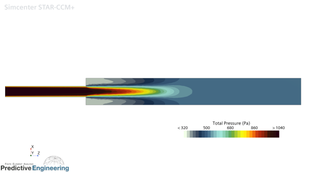
A better way to present this data is to use the Total Pressure. The total pressure will sum the static, dynamic and hydrostatic components. What will be left is the expected decrease in pressure with flow direction due to losses
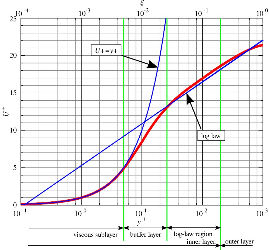
Your colleague is performing a heat transfer analysis using the All Y+ Realizable K-Epsilon turbulence model. You see their plot of wall Y+ values on the surface, which shows significant portion of values between 10 to 25. Would you believe their analysis results?
NO. The All Y+ turbulence models in major commercial codes seek to bridge the gap between directly modelling the viscous sublayer, or using a logarithmic wall function, in the outer log-law region of the boundary layer. This Y+ value is a dimensionless number that is determined by the distance of the1st cell to the wall, frictional velocity, and kinematic viscosity (similar to a local Reynolds number). Y+ values less than 5 show the cell is in the viscous sublayer region next to the wall. Y+ values above 30 state a logarithmic wall function can be used to estimate the flow. In between these values is a no-mans land. This is a buffer layer where commercial codes implement a smoothing function to bridge these two regimes together. This allows CFD engineers to model complex flow through complex geometries where it would be nearly impossible to create a mesh that completely falls in either the viscous sublayer or log-law region. Having small areas that fall within the buffer layer using the All Y+ methods is sometimes unavoidable, but if a significant portion of the model is in this region, the results will be severely compromised.
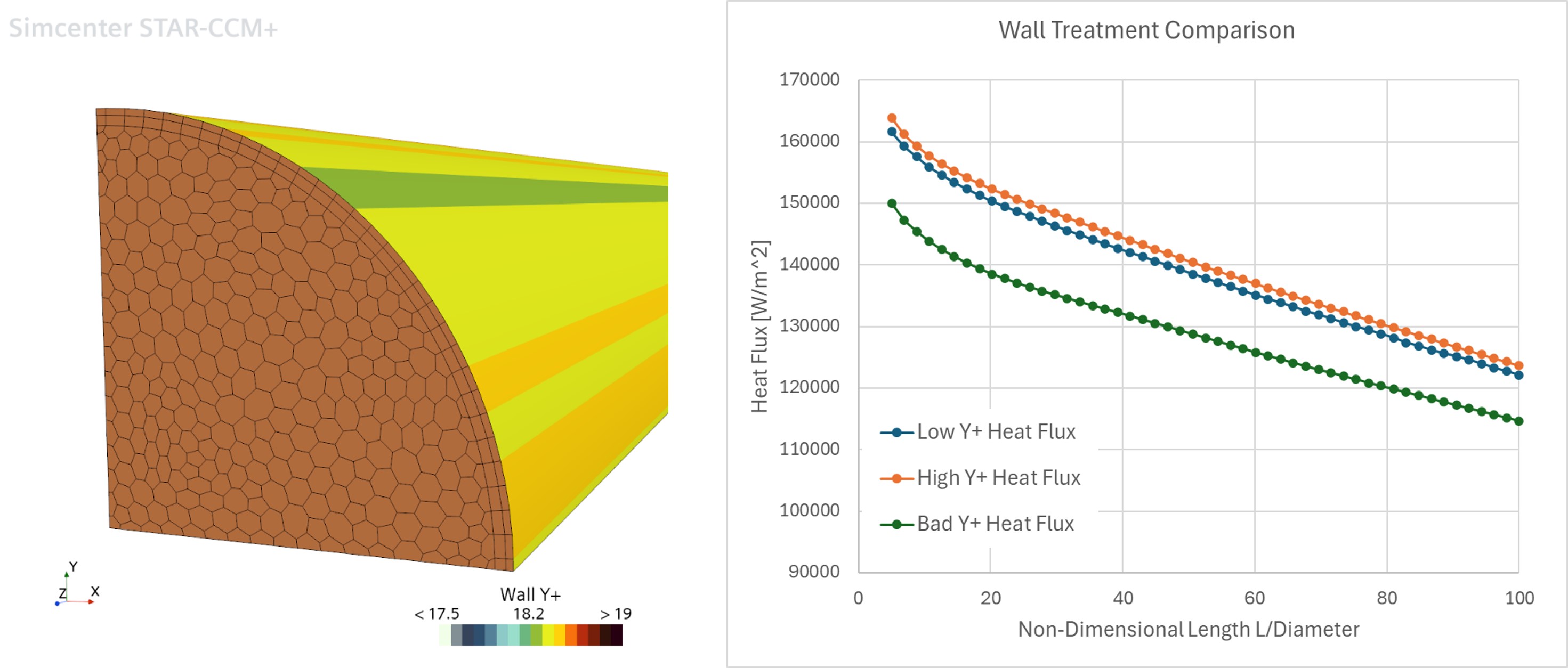
To demonstrate the impact of what a poor mesh could have on your thermal results, we re-ran the study presented by Siemens in their support article comparing the impact of wall functions on thermal results, but we add in a third case with a poor choice for Y+. This is a simple case of flow down a tube with a constant wall temperature. We see the wall functions lead to a 1% to 2% over prediction of heat flux, which is a manageable difference. In comparison, the poor choice in Y+ leads to a significant error of under predicting the heat flux by 5% to 10%. For small regions within a model, this impact will be negligible on the final solution, but if these values represent a large portion of the model, delete the result and start over.
For an implicit transient solution, with a segregated solver, you must keep your CFL value less than 1.
- True
- False
False. The CFL (or Courant number) is the ratio of analysis time step to the time it takes the fluid to travel across the width of the cell. For an explicit analysis, this value must be less than 1 for all cells (i.e. the fluid never fully transverses the cell during a time step). With implicit schemes, that utilized inner loop iterations to solve for a particular time step, these values can be greater than 1 to speed up the solution time. Average values of up to 5 or 10 can be achieved, but this still depends on the overall dynamics of the flow. For highly dynamic flow, we would suggest trying to keep the CFL value close to or below 1.
To demonstrate this capability, we performed a laminar vortex shedding analysis with different time steps, as seen in the video below. The timesteps result in maximum CFL values of 1, 2, and 6 respectively. This is a fairly dynamic problem, and we are able to get solutions for all time steps using the implicit solver. The larger time step with a CFL of 2 provides a pretty close comparison to the suggested solution method, but as we get the time step much larger, where the maximum CFL value is 6, we start to see a significant amount of numerical diffusion.