LS-DYNA: Observations on Material Modeling
This is the 4th in a series of informal articles about one engineer’s usage of LS-DYNA to solve a variety of non-crash simulation problems. The first was on LS-DYNA: Observations on Implicit Analysis, the second was on LS-DYNA: Observations on Composite Modeling, and the third was LS-DYNA: Observations on Explicit Meshing.
As a former metallurgist whose specialty was structure-property relationships, I have a keen appreciation for how materials deform under load. At the federal lab where I worked, we had a lot of mechanical test equipment where I could break, crush and impact all sorts of things. This experience grounded me in my appreciation of how difficult it is to simulate the mechanical response of materials using some sort of X-Y plot of stress versus strain.
If one has been reading my prior articles, one knows that I obsess on error management. One client remarked, “Could you put error bars on your stress numbers?” I wish I could, but we do engineering projects that have tight schedules and finite budgets. To really quantify your model’s error, or perhaps better said, its deviation from experimental truth, requires one to start first with the material model and then move along through all the other modeling assumptions and slights of hand. One day I’ll find my Unicorn client that wants to do this but I’m not holding my breath. In the meantime, for us working engineers, let’s talk about simple material modeling that will keep you out of the weeds (since for the difficult stuff I punt and hire a real ‘DYNA material expert).
General Entry-Level Discussion on Material Modeling
Everybody’s Favorite: HSLA Steel
If you are looking for a primer on how to convert engineering stress v strain into true stress v strain, you have come to the wrong place. That’s too simple and enough academicians have already covered it in detail. So let’s talk about some of the tricks of the trade that I have learned from reading and my colleagues. A quote that I just love to repeat is “A piece of paper with a stress v strain curve on it is NOT material test data.” That is, one starts with real experimental test data in spreadsheet form and not picking points off of a curve with a straight-edge and pencil. Once you have real data, it can be imported into one of the world’s handiest material test data processing free software – LS-PrePost (LSPP). With your data in LSPP, you can average it to remove little spikes and then with the reduced data (one saves the averaged data and then reads it back into LSPP), one can take the derivative to find slope changes. Since steel deforms in a smooth continuous manner through dislocation movement, one should find no sharp slope changes in the curve.
If you do – go back and do some more averaging. Once you have a smooth curve, you can then convert it to true stress versus strain. Also keep in mind that LS-DYNA discretizes your curve down to a default 100 points (see Remark 1 in *DEFINE_CURVE writeup). For basic steels this is fine but for most rubbers/foams/bone/etc. it is useful to bump this value up to say 500 (see LCINT in *CONTROL_SOLUTION) since the curve goes from compression to tension and is highly nonlinear. What this means is that when you are smoothing your material data, there is rarely a need to have a ‘DYNA material curve with more than 500 XY pairs.
For metallic materials, a better way is to use an equation and avoid this whole messy point-to-point interpolation. A good choice is the *MAT_SIMPLIFIED_JOHNSON_COOK (*MAT_098) for numerical efficiency and, an even better reason, that Varmint Al has compiled a list of 1,044 metallic materials such as aluminum, copper, magnesium, steel, stainless steel, etc. all ready to drop into your ‘DYNA model.
What about Strain Rate for Steels?
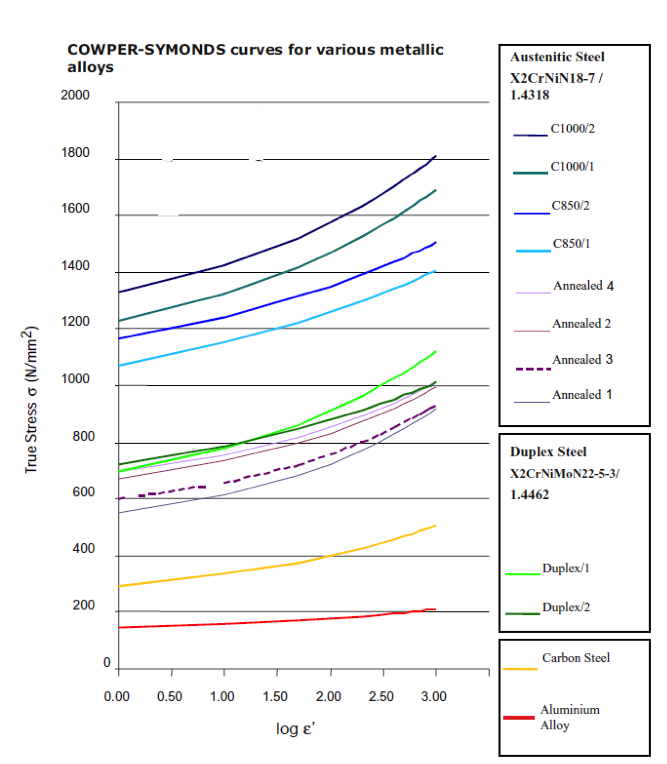
Most ‘DYNA simulations are dynamic, meaning that the yield stress will scale (i.e., increase) with the strain rate (see Figure 1). This, of course, is a generality and unless you have published or experimental data, it is a bit of guess work. It is not something to run from; just realize that if you have a high-strain rate event, you might want to play around with strain rate effects.
Figure 1: Strain rate effect in steel and aluminum
Material Failure Modeling: GISSMO et al.
I would be remiss not to say a few words about Generalized Incremental Stress-State dependent damage Model or GISSMO (I know – it doesn’t exactly match up) that is setup under the *MAT_ADD_EROSION card. Let me say that if you think you need to use GISSMO it might be a good time to hire a ‘DYNA material modeling expert and that is not me.
My observation on GISSMO is that it allows one to account for triaxial stress effects and facilitates a more accurate prediction of material failure. My more basic approach is to differentiate between tensile and compressive failure modes. This can be done by using EFFEPS to define compressive failure strain and MXEPS to define tensile failure. I like to use a ratio of 3-to-1 between EFFEPS and MXEPS. Why? Lots of reasons due to compressive failure in metals, but as a mechanician I like to explain the use of this 3-1 ratio based on the stress concentration factors for a hole in an infinite plate.
Under compressive load, a tensile stress of +1 exists at the 0 degrees (aligned with the load) and a compressive stress of -3 at 90 degrees and of course, vice-a-versa for a tensile load. Thus, under compressive load, all defects and voids in the material will have tensile stresses equivalent to yield at 3x compressive loads – to a general back-of-the-envelope degree.
One can also desensitize the failure behavior by requiring all integration points in the element to fail prior to element deletion (NUMFIP) and so on and so forth. The number of options is truly amazing and scary. Before getting lost in the bark and not seeing the forest, accurately predicting material failure can be crazy complex and it requires companion studies on mesh sensitivity, element choice (plate v solid), element formulation, hourglass, contact formulation, mass scaling (come on – everybody uses a bit of mass scaling) and I’m sure more stuff.
My approach is to keep it simple going out of the gate and just use EFFEPS and MXEPS. For our simulations over the last decade, it has served us well with accurate predictions but since all models are wrong, your experience may be different from ours.
The Softer Side of Material Modeling: Plastics / Elastomers / Foams
Let’s get it out on the table, *MAT_PIECEWISE_LINEAR_PLASTICITY (*MAT_24) does a really nice job in capturing the deformation response of engineering plastics. One just has to be careful with how you define the stress v strain curve (understatement). As for elastomers (rubbers) and foams, I have relied upon *MAT_SIMPLIFIED_RUBBER/FOAM (*MAT_181) and *MAT_FU_CHANG_FOAM (*MAT_83), respectively. What I like about *MAT_181 and likewise with *MAT_83) is that one can enter experimental force versus elongation data directly into the material card and be done with it.
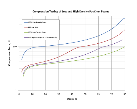
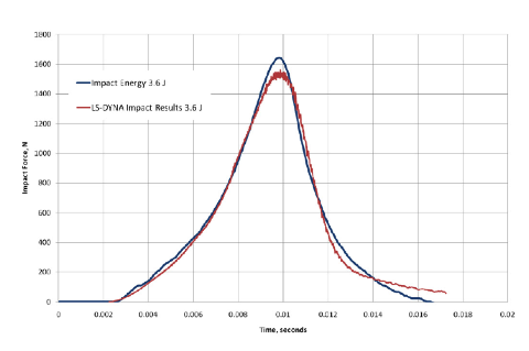
In Figure 2, I show some test data and its comparison to experimental results. There is a funny story behind this project. For several long days I labored to get correlation between the model and the test. The test’s peak impact force was far higher than my model. After suffering enough, I called my material expert and expressed my plight.
He asked how the experimental data was being processed and I said that they were averaging the data over several impacts. There was a long pause and then the obvious was spoken. If the impact is sufficiently severe, the foam walls will break down and the foam crushes into a dense brick of plastic. Hence, the peak force would, of course, steadily increase after each impact. I went back and used only the data from the first impact event and the model correlated to engineering perfection (i.e., 5%).
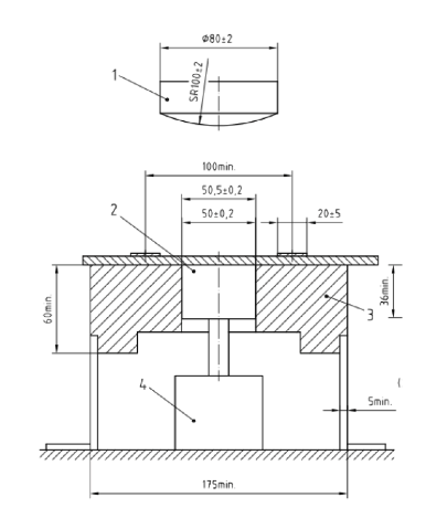
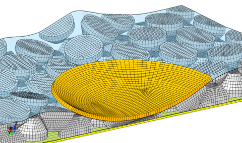
Figures 2a-2d - Foam Material Modeling for Impact Analysis
Experimental Foam Data:
EN‐1621‐2 Impact Test
LS-DYNA Impact Analysis of Foam Model
Comparison of Impact Test Data with FEA
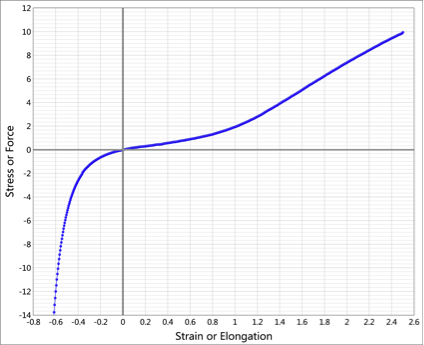
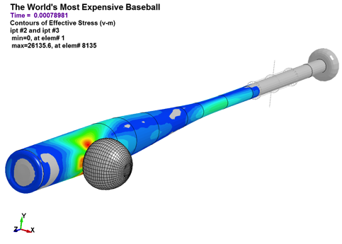
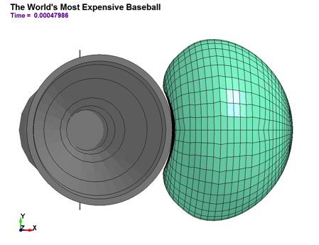
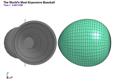
Before leaving material modeling of soft stuff, I want to show a really sweet *MAT_181 curve for an elastomer. Such a curve was used for modeling a baseball. It was a nice little project where the cost to model the bat was a few thousand but the cost to calibrate the material model to match a “baseball” was in the tens of thousands. Why so much? The bat was simple aluminum but the complex response of a baseball under large deformation was a whole other ball game. Figure 3 shows the material curve and a few freeze-frames of the ball’s response.
Figures 3a-3d: *MAT_181 is handy for all sorts of complex soft materials
The Cutting Edge: Composite Material Modeling
We tend to advocate getting good with one material model and then sticking with it unless some dire emergency requires something different. Under this banner, *MAT_ENHANCED_COMPOSITE_DAMAGE (*MAT_54) is hard to beat. As for damage prediction in composites, it is a very complex subject and a prior blog covers some of the challenges around composite modeling. On our work, we just stick to using fiber failure strains and avoid touching the concept of interlaminar failure and fiber debonding. There are a couple of reasons for this basic approach: (i) Our work uses plate elements and (ii) in failure, once the outer fibers start to pop, the only thing that holds the composite structure together is a bit of weak epoxy or for sandwich materials, the foam core. If one is interested in damage tolerance over multiple cycles, it is a bit of a quasi-research project.
My Cookbook Recipe for Material Modeling
Enough with generalities. Here’s the cookbook recipe for when I have to create my own material curve from experimental data. I start with a LS-DYNA model of the test setup and input my true stress v strain or force v elongation curve. Often times I’ll run the analysis in both implicit and explicit, just be sure everything is working as advertised. To verify your material model, take the force versus elongation output and overlay it on your original spreadsheet data. Of course, this may seem a bit odd at first but remember that experimental stress v strain data is engineering stress v strain data and that the cross-sectional area is constant and that one starts with a known sample length. Thus, your ‘DYNA results of force versus elongation should overlay perfectly your experimental data.
If You Would Like to Get Better at Material Modeling
I would suggest three things: (i) Read with a critical eye and check out the authors background whether they are engineers solving problems or academicians generating CV bullets; (ii) Get experimental test data and do your own material model generation and (iii) Attend FEA material modeling classes given by industry experts.
Running for the Door
For now, I have exhausted my current list of bloggable items of interest from implicit analysis, composite modeling, explicit meshing and now general material modeling. I know that other topics surely await but for now, this is what I’ve got. I hope you have enjoyed my blog and maybe in six months or so something else will come up.